Fashion Classifier with CNN using Keras

Hello and welcome! Whether it’s your first time here or you’re a regular reader, I appreciate you taking the time to engage with my blog :)

The goal of this project is to take my first steps in deep learning by building a Convolutional Neural Network (CNN) image classifier using Keras. However, it does not delve into other essential aspects of a data science pipeline, such as data gathering (scraping, etc.), cleaning, deployment, etc. I have covered these aspects in my ‘Likelihood of Crowd Funding Success’ project, which I have previously shared here

1. Introduction

In the realm of computer vision, one of the most exciting and impactful applications is image classification. In this blog, we’ll embark on a journey to create a CNN image classifier using Keras. Our dataset of choice? The Fashion MNIST dataset, which is a benchmark similar to MNIST based on fashion products, and was donated by Zalando to the AI research community.

The link to the Jupyter Notebook shared in GitHub is here.

2. Understanding the Fashion MNIST Dataset

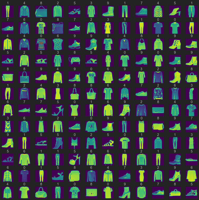
Fashion-MNIST dataset serves as a substitute for the popular and original MNIST dataset, but instead of handwritten digits, it consists of small images of fashion items. Commonly employed for image classification benchmarking and educational purposes, this dataset comprises 10 classes, each representing a distinct fashion item. The goal is to classify each image into one of these mutually exclusive categories:

• 0: T-shirt/top
• 1: Trouser
• 2: Pullover
• 3: Dress
• 4: Coat
• 5: Sandal
• 6: Shirt
• 7: Sneaker
• 8: Bag
• 9: Ankle boot

Each grayscale image is 28x28 pixels, with pixel values ranging from 0 to 255, indicating grayscale intensity. The dataset encompasses 60,000 training images and 10,000 testing images and is typically formatted for easy integration into machine learning frameworks. Fashion-MNIST serves as a challenging benchmark for evaluating machine learning models, particularly in the realm of image classification tasks, surpassing the original MNIST dataset by presenting more complex and diverse images. Introduced as a replacement for MNIST, Fashion-MNIST addresses the limitations of the latter by providing a more realistic representation of challenges in image classification tasks.

3. Importance of Convolutional Neural Networks(CNN)

Convolutional Neural Networks (CNNs) have emerged as a revolutionary technology, particularly in the realm of image classification within the domain of deep learning. While traditional neural networks possess the ability to automatically learn patterns and representations from data during the training process without human interventions like feature engineering, they encounter challenges with image data due to its high dimensionality and spatial dependencies. CNNs address these challenges through specialized convolutional layers that capture local patterns and spatial hierarchies.

The architecture of CNNs is designed with layers, and each layer focuses on learning specific features. Early layers may capture simple features like edges and colors, while deeper layers delve into more abstract and complex features, such as shapes or high-level patterns. This hierarchical representation allows the network to understand and recognize increasingly sophisticated concepts as information flows through the layers. In essence, this architecture mimics the human visual system, where early layers detect simple features like edges and textures, and deeper layers recognize more complex and abstract representations.

The integration of deep learning principles within CNNs has significantly advanced image classification, achieving state-of-the-art results in various benchmark datasets. Their robustness to variations in scale, orientation, and lighting, coupled with powerful transfer learning capabilities, enables CNNs to generalize well to diverse real-world scenarios. As a result, CNNs have become commonplace in critical fields such as medical imaging, autonomous vehicles, and more, showcasing the transformative impact of deep learning on image analysis and understanding.

4. Libraries Used

Python 3.8.18 was employed within the Anaconda environment.

Key libraries used were: Matplotlib, TensorFlow, Keras, NumPy, Scikit-Learn’s metrics module, and Seaborn for visualization

5. Data Preprocessing:

Preparing the data is a critical aspect of any machine learning project. Preparing the data for training involves preprocessing steps like resizing images (not required for this dataset since all our images are 28 x 28), normalizing pixel values, and splitting the dataset into training and testing sets. These steps ensure that the model learns effectively and generalizes well to new, unseen data.

Loading and Splitting Dataset to Training and Test Data

# Use the following lines of code to get the dataset and  split into training and test:
import tensorflow as tf
(X_train, y_train), (X_test, y_test)= tf.keras.datasets.fashion_mnist.load_data()

Normalizing the data involves converting pixel values from a range of 0 to 255 to a range of 0 to 1. While this step is crucial when dealing with features of varying scales, for this dataset, it is considered an optional step because each pixel of the images already exists within the same range of 0 to 255.

Normalizing the Data

x_train = x_train.astype('float32') / 255
x_test = x_test.astype('float32') / 255

One-Hot Encoding the Target Classes

The target class data (y_train, y_test) is in integer form (0 to 9), this has to be preprocessed to one-hot encoded labels:

number_cat = 10 # 10 categories or classes in our data
#converts y_train to matrix with 0s, and 1s with number of columns equals classes
y_train = tf.keras.utils.to_categorical(y_train, number_cat)  
y_test = tf.keras.utils.to_categorical(y_test, number_cat)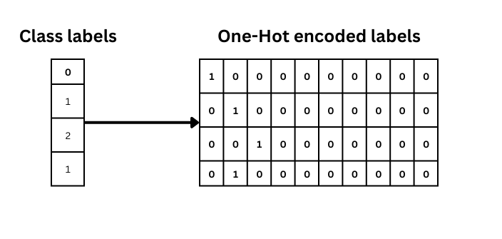

Reshaping: Creating Grayscale Color Channel Dimension

Convolutional Neural Networks (CNNs) expect input data to have a color channel dimension, even if it’s grayscale. This step ensures that the input data has the correct shape for CNNs. This is done as follows:

X_train = np.expand_dims(X_train, axis=-1)
X_test = np.expand_dims(X_test, axis=-1)

This should reflect in as a change of shape of X_train from (60000, 28, 28) to (60000, 28, 28, 1).

For smaller datasets, additional steps may be needed e.g. data augmentation via applying random transformations (rotations, flips, zooms, etc.) to the training images to help improve model generalization. Now with these steps done, the data is pre-processed and ready to build a CNN Model.

6. Building the CNN Deep Learning Model:

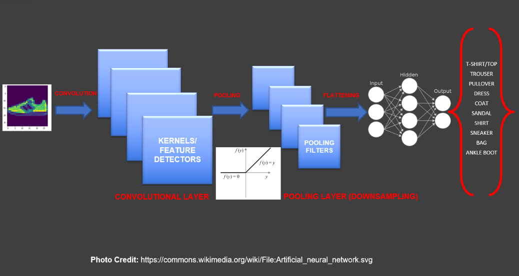
CNN differ from traditional neural networks in that there are additional layers, specifically kernel and convolutional layers, which act as feature detectors. These detectors in the kernel and convolutional layers are adept at identifying and extracting diverse features from input images like edges, textures, or shapes. Each filter focuses on recognizing a specific pattern. When the filters scan the entire image, they create maps highlighting where certain features are present. These are called feature maps. To simplify the information (reduce dimensionality) and make it more manageable, often pooling layers are used. They reduce the size of the feature maps by keeping only the most important information e.g. in max pooling, for each region of the input (e.g., a 2x2 window), the maximum value is selected and retained in the output while the other values are discarded. By downsampling the spatial dimensions, pooling layers reduce the amount of information in each feature map, making it computationally more efficient. After convolution and pooling, the information is flattened into a single line of numbers. This prepares the data to be used in the traditional neural network layers. The entire process, from detecting basic features to making complex predictions, is done in a hierarchical way. Simple features are detected first, and then more complex patterns are built on top of them.

Defining the CNN Model

In Keras there are two APIs for defining a model: Sequential model API and the Functional API. In this project, we have used the Sequential model API, which easily allows to add layers in a step by step fasion. This is a convenient way to quickly build simple models where the data flows sequentially through each layer.

Our CNN model comprised three convolutional layers. The first two layers included max-pooling, while the last layer consisted of flattening layers. Each of these layers uses the ‘relu’ activation function, defined as f(x) = max(0, x). This function is applied element-wise to each element in the input tensor. Essentially, the purpose of ‘relu’ is to introduce non-linearity into the system and to simplify it. Non-linearity is crucial in neural networks because it enables the network to learn complex patterns and relationships in the data. In addition to the convolutional layers, the model includes two dense neural layers, with the final layer comprising 10 neurons to map to the 10 target classes.

from tensorflow.keras import datasets, layers, models

# networks are built from left to right sequentially
cnn= models.Sequential()
#32 filters, each filter size is 3 x 3, activation function 'relu', rectified linear units
# relu sets negative to zero, while keeping positive as same, basically introduces non-linearity to system
cnn.add(layers.Conv2D(32, (3,3), activation ='relu', input_shape=  (28, 28, 1))) 
cnn.add(layers.MaxPooling2D(2,2))

# Unlike the generic image shown from wiki, it is possible to add another convolutional layer and pooling as well
cnn.add(layers.Conv2D(64, (3,3), activation ='relu')) #input shape automatically taken from previous layer
cnn.add(layers.MaxPooling2D(2,2))

cnn.add(layers.Conv2D(64, (3,3), activation ='relu')) #input shape automatically taken from previous layer
cnn.add(layers.Flatten())

cnn.add(layers.Dense(64, activation= 'relu')) # dense neural network layer, 64 neurons

# output layer, since only 10 classes of output
# softmax output layer, converts input vector of real numbers to classes of probabilities
# output between 0 and 1, all 10 neurons outputs add to 1, so if first neuron is majority, then classified as class 1  
cnn.add(layers.Dense(10, activation= 'softmax'))
cnn.summary()

7. Training and Evaluating the Deep Learning Model:

With the model architecture in place and data preprocessed, we can train the CNN using the training set and validate it using the validation set. Monitoring metrics such as accuracy and loss (loss function: crossentropy for classification problems, with ‘categorical_crossentropy’ for multi-class problems) during training provides insights into the model’s performance.

# compiler needs the optimizer to be specified, RMSprop is neural network training optimizer that is adaptive
# loss used is for multi category class, for binary classification problems use binary_crossentropy
cnn.compile(optimizer = tf.keras.optimizers.RMSprop(0.0001, decay = 1e-6), loss ='categorical_crossentropy', metrics =['accuracy'])

The training phase involves feeding the prepared dataset into the CNN and adjusting the model’s weights internally to minimize the ‘categorical_crossentropy’ loss function. After training for 10 epochs, and with a batch_size of 512 (no of images fed at once to the neural network), the accuracy achieved on training data was 87.7%.

epochs= 10 # iteration/run for training of neural network
# batch_size of 512 is no of images feeding in at once to train
history = cnn.fit(X_train, y_train, batch_size= 512, epochs= epochs) 

The accuracy achieved on the test data ~ 85% was similarly high and close to the training data accuracy indicating that the model generalized well without any siginificant overfitting.

cnn.evaluate(X_test, y_test)

Visualizing the Predictions

For visualizing the test data predictions, predicted_classes were evaluated from the model using the test data.

predicted_classes = cnn.predict(X_test)

Because the predicted classes would also have the structure of the target y (previously, one hot encoded to consist of 10 columns corresponding to each class), they were converted to a 1-D array format using the following code:

predicted_classes=np.argmax(predicted_classes,axis=1) # the max argument corresponds to the class chosen
y_test = y_test.argmax(1)

Refer to Jupyter notebook for detailed code

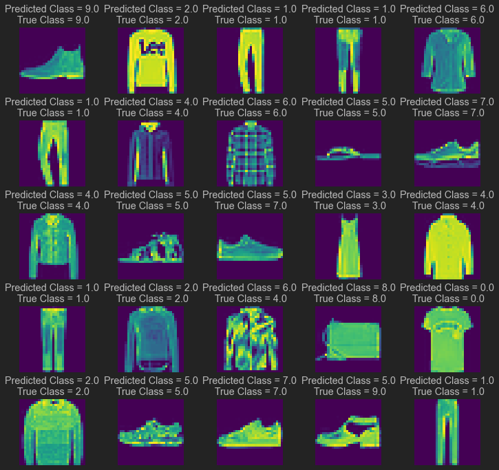
We then visualized a 5x5 grid of fashion item images from the test data, showcasing both the predicted (predicted_classes) and true classes (y_test) as shown below:

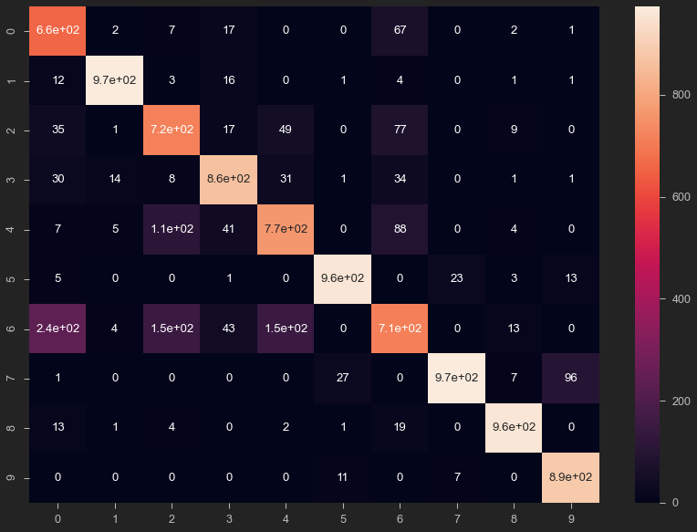
Understanding Misclassifications

Additionally, we explored the confusion matrix, revealing interesting patterns. Notably, around 150-250 images from class 6 (shirt) were wrongly predicted as class 0 (T-shirt, top), class 2 (Pullover), and class 4 (Coat). Similarly, about 110 entries from class 4 (Coat) were misclassified as class 2 (pullovers). These misclassifications by the model intuitively make sense, as these are all upper body wear and visually similar compared to trousers or sneakers. 96 images of Sneaker (class 7) were wrongly misclassified as Ankle boot (class 9), both being closed footwear in contrast to only 27 images misclassified as sandals, which is open and relatively more visually distinct. Interestingly, the same magnitude of misclassification is not seen in the reverse i.e. very few Ankle boot (7 images) were misclassified as sneakers. This is reflected in the lower precision of class 7 (sneakers) ~ 88%, relative to much higher, 98% precision of class 9 (Ankle boots).

import seaborn as sns
from sklearn.metrics import confusion_matrix
cm= confusion_matrix(predicted_classes, y_test)
plt.figure(figsize= (14, 10))
sns.heatmap(cm, annot= True)
# model predictions as the rows, versus the ground truth (y_test)
# whenever model predictions match y_truth, the diagonals capture that
# non-diagnonal are wrong predicted cases 

x-axis: predicted classes; y-axis: true classes

from sklearn.metrics import classification_report
num_classes = 10
target_names = ['class {}'.format(i) for i in range(num_classes)]

print(classification_report(y_test, predicted_classes))


                precision    recall  f1-score   support

           0       0.87      0.66      0.75      1000
           1       0.96      0.97      0.97      1000
           2       0.79      0.72      0.75      1000
           3       0.88      0.86      0.87      1000
           4       0.75      0.77      0.76      1000
           5       0.96      0.96      0.96      1000
           6       0.54      0.71      0.62      1000
           7       0.88      0.97      0.92      1000
           8       0.96      0.96      0.96      1000
           9       0.98      0.89      0.93      1000

    accuracy                           0.85     10000
   macro avg       0.86      0.85      0.85     10000
weighted avg       0.86      0.85      0.85     10000

8. Conclusion:

In this blog post, we’ve explored the journey of building a CNN image classifier using Keras on the Fashion MNIST dataset. From understanding the dataset to constructing the model architecture, preprocessing data, and evaluating the model, this project serves as a quick starter hands-on guide for anyone venturing into the world of image classification in data science.

Our model achieved an accuracy of 85% on the test data, highlighting the potential of a simple CNN architecture on the Fashion_MNIST dataset. Hyperparameter tuning was not pursued with much depth in this project and remains as an area for further exploration. Moving forward, an exciting avenue for improvement involves scraping classified images from e-commerce platforms like Amazon. This would present exciting data preprocessing learning challenges, such as resizing images of different sizes, addressing class imbalances, handling color images, managing varying backgrounds, images with different camera angles, and addressing hierarchical encoding, among others.

In conclusion, this project served as a valuable learning experience in building and evaluating a CNN model.